
The Mathematics of Sound and the Search for Negative Peaks
CliDeck Research Notes · Bass Plus · 18 October 2026
Abstract
How far below its average must a collection of synchronized waves fall? This question leads from a simple model of sound to Chowla's cosine problem, a difficult question about sums of distinct integer frequencies. This report brings together a sequence of ninety exploratory approaches, their mathematical checks, and their limitations. It develops exact examples, a spectral interpretation, a counterexample to minimum detection by a natural sampling grid, and an explicit approximation bound whose sufficient polynomial degree depends on the number of frequencies and the requested error, but not on the largest frequency. The approximation method belongs to Lasserre's established pushforward measure hierarchy; its Chebyshev filtering mechanism is closely related to work of Slot and Laurent. We claim neither a solution of Chowla's conjecture nor priority for this general method. The useful outcome is a reproducible account of what can be proved, what finite computations show, and which tempting extensions fail. Eight figures connect the analysis to phase locking, sampling, weighted amplitudes, spectral bands, and finite searches.
1. The question behind the waves
Take a finite set of distinct positive integers , and let . We study the real function
Every component has amplitude one. Every initial phase is zero. There is one common variable : the components cannot choose their phases independently. Define the depth of the most negative excursion by
Chowla's question asks whether there is an absolute constant such that
for every such set . The constant would have to work for consecutive frequencies, sparse frequencies, sets with strong arithmetic relations, and arbitrarily large frequency values. There is no upper bound on in the question. Recent papers make substantial progress on weaker polynomial lower bounds, but the sources consulted for this report continue to distinguish that progress from the square-root target. JMTZ2025 Bedert2026 Shankar2026
The quantifiers are the heart of the problem. Finding a large negative excursion for a particular set is valuable, but proving it for every finite set is a different task. Replacing by the set-dependent number is an exact description, not a resolution: one must still prove that the infimum of this function stays positive over all sets and all sizes.
For a sound interpretation, set , where is a base frequency in hertz. Then the physical frequencies are . The mathematical model describes an ideal harmonic signal with equal amplitudes and synchronized phases. Music and equalized audio usually have unequal amplitudes, changing phases, noise, and finite observation windows. The model helps explain interference and measurement; it does not, by itself, establish a benefit of an audio product.
2. What the coefficient means physically
Use normalized averaging over a full period:
Orthogonality gives and . Thus the root-mean-square amplitude is , while . All signals in this model have the same RMS amplitude when they have the same number of frequencies. Their negative peaks can nevertheless differ.
For example,
For the first set, put and complete the square:
For the second, both cosines equal at . The first signal has a shallower trough despite identical RMS amplitude. The dimensionless negative crest factor is
This explains the normalization: would be a uniform lower bound on a normalized negative peak. It is not an energy quantum, a material constant, or a new universal constant of physics.
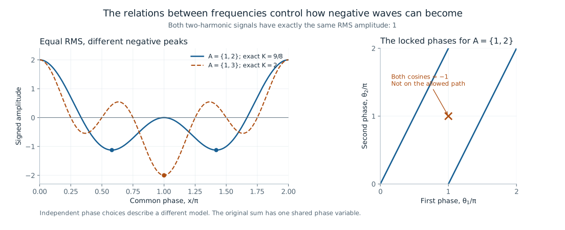 Figure data (JSON) · SVG · PNG
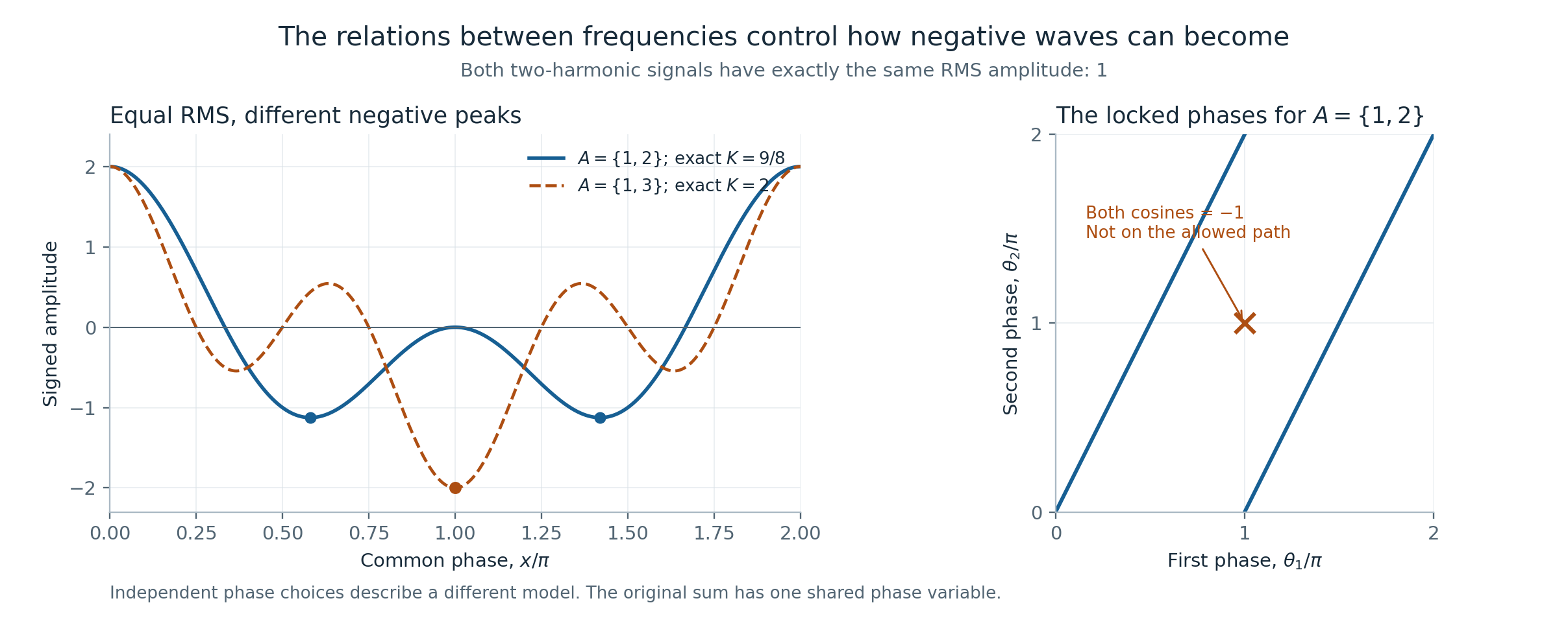
Figure 1. Phase locking changes the attainable trough. The two signals have equal RMS amplitude. For , the hypothetical independent-phase value is inaccessible; the exact common-phase minimum is . The chart keeps the hypothetical model explicitly separate from the actual signal.
Explore interactively
If represents acoustic pressure relative to equilibrium, negative values describe rarefaction. They do not mean negative acoustic energy. In the plane progressive-wave approximation, average intensity is proportional to mean-square pressure, with proportionality determined by acoustic impedance. This physical distinction matters whenever a proposed proof replaces a signed wave amplitude by a squared magnitude. BakerAcoustics
3. Why a single common phase is restrictive
The vector follows a one-parameter path. For multiple frequencies, it does not explore the entire cube . For , the relation prevents both coordinates from being at once. Allowing separate phases removes that constraint and changes the problem.
The same point becomes geometric with three frequencies. The path
is a curve inside a cube. Colouring each point by the sum of its coordinates shows exactly which signal values this shared clock can reach. A rotation of the display changes our viewpoint, not the set of attainable states. This is why a three-dimensional figure is useful here: its geometry represents an actual constraint.
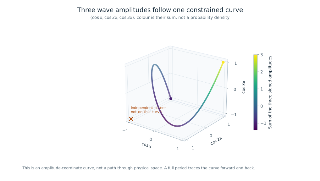 Figure data (JSON) · SVG · PNG
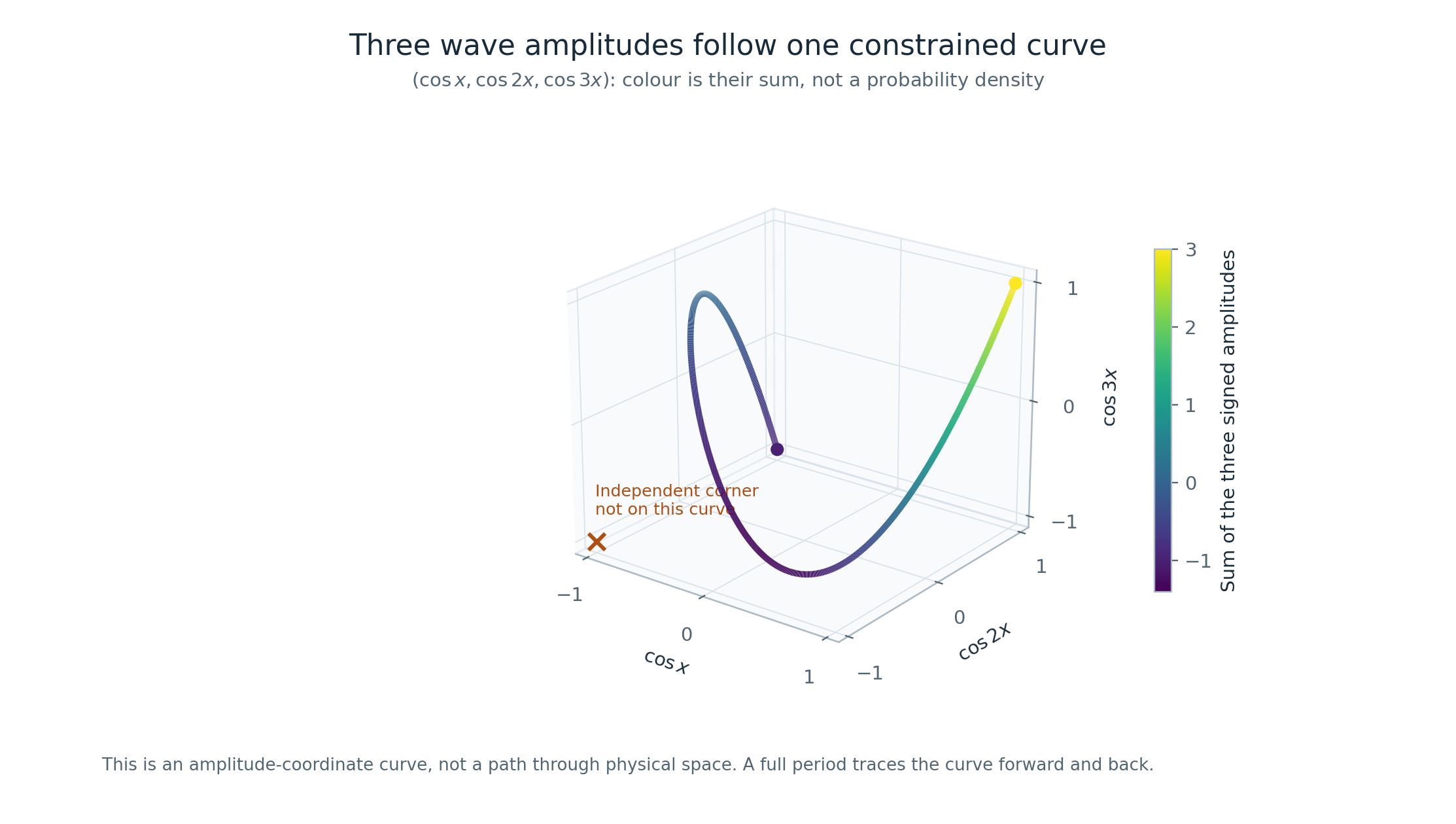
Figure 2. One clock traces a curve, not a cube. The colour is the actual sum . The corner is not on the curve. Over a full period, the real cosine-coordinate curve is retraced. The figure is a classical phase model, not a visualization of a quantum state.
Multiplying every frequency by the same positive integer has a different effect. Since , it compresses the pattern in time while preserving its full-period range:
A trough can become narrower in a local time window without becoming shallower. Any argument that estimates the total negative contribution from one local width must account for the increased number of repeated troughs.
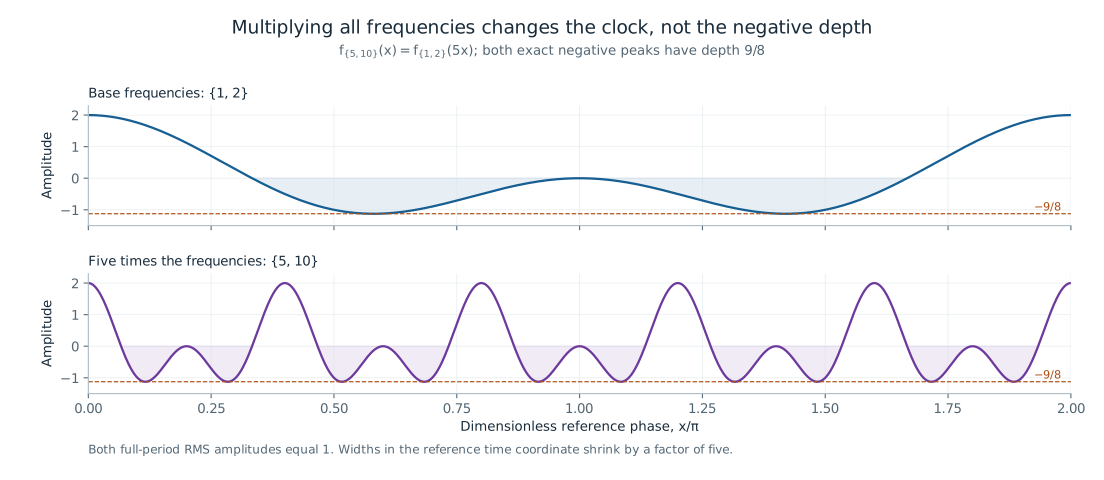 Figure data (JSON) · SVG · PNG
Figure 3. Frequency scale and peak depth are different quantities. The sets and both have . Dilation produces more oscillations within the same displayed interval. It does not improve the normalized negative minimum.
4. A sampling grid can hide the trough
Consider and let . On the equally spaced grid , a roots-of-unity identity gives
The grid therefore reports a negative depth of only . It also reports the correct mean-square value:
Yet at the point between grid locations , the Dirichlet-kernel identity yields
Consequently,
The hidden excursion grows linearly with . This is an exact family of counterexamples to using the smallest raw sample as the true minimum. It is not a failure of trigonometric interpolation: the same grid contains enough information to reconstruct this finite-bandwidth trigonometric polynomial. Reconstructing a signal and simply taking the smallest of its stored samples are different operations.
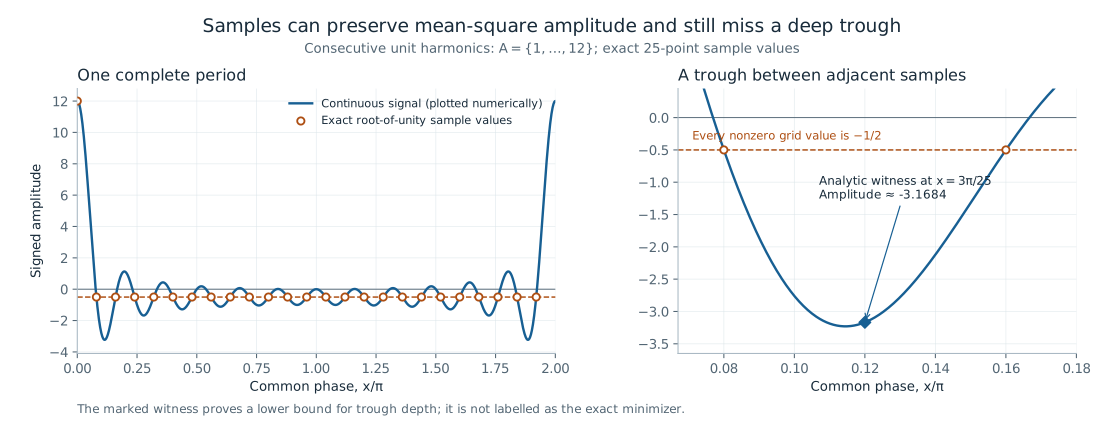 Figure data (JSON) · SVG · PNG
Figure 4. Correct RMS does not certify the minimum. For and , every nonzero sample is , while the continuous curve passes much lower between samples. The highlighted off-grid point is an exact witness. The drawn smooth curve is an illustration, not a substitute for the identity.
A simple rigorous guard is available for a general set. For a grid with equally spaced points, let be minus the smallest sample. The derivative bound gives
A second-derivative argument at a true minimum improves the error bound to when that is smaller. A scientific interactive chart should display the certified interval alongside the sampled value. A dense curve by itself does not supply a certificate.
5. The same function as a lattice spectrum
There is an exact way to reinterpret the cosine sum as a particle-like hopping model. Let be the bilateral shift on square-summable sequences indexed by the integers, and define
Fourier transformation turns each shift into a complex phase. The operator becomes multiplication by , so its spectrum is the full interval
This is a mathematical identity. The wave minimum becomes the lower edge of the spectrum of a translation-invariant lattice operator. The model is related to tight-binding descriptions of hopping on a lattice. An infinite lattice can have continuous spectral bands even though its sites are discrete; discrete position labels alone do not quantize all possible energies. TongAQM
A finite ring introduces a boundary condition. With sites and a phase twist , its eigenvalues are
At , the ring sees one sampling grid. As varies through a full turn, the eigenvalue curves sweep the entire continuous phase variable. Taking the minimum over both and recovers exactly. The boundary twist repairs this finite model's missing phases; it does not create a new universal lower bound. Twisted boundary conditions are an established tool in spectral physics. Bardyn2014
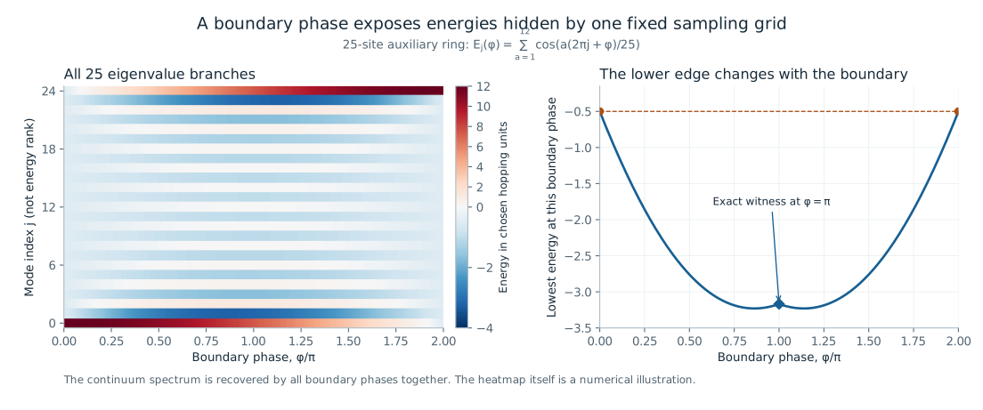 Figure data (JSON) · SVG · PNG
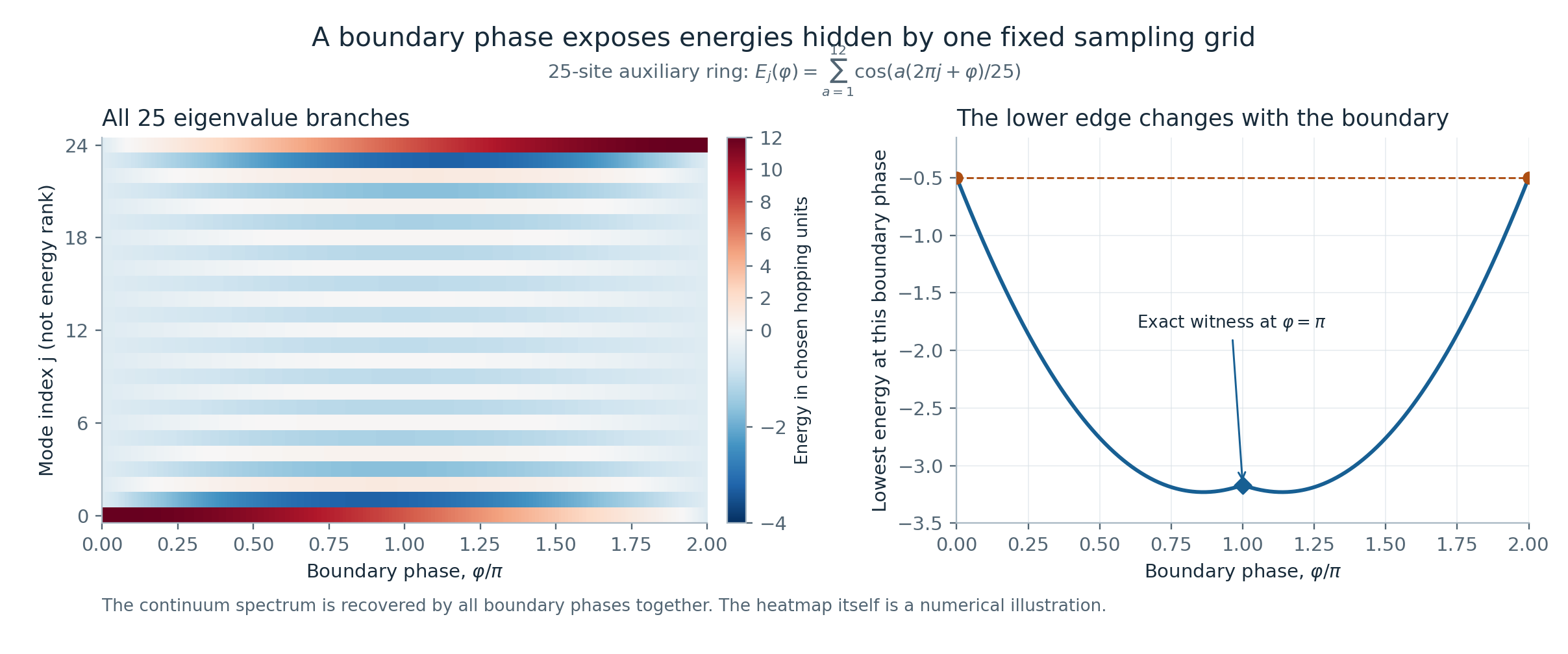
Figure 5. A boundary phase reveals what one finite ring misses. The heatmap shows the actual values for and . The untwisted column has the exceptional two-value spectrum, while other twists expose lower energies. The vertical coordinate labels finite eigenvalue branches rather than an independent sound frequency.
6. A certified way to approximate each minimum
For a real polynomial of degree at most , consider the weighted average
The denominator is positive for nonzero because is nonconstant and its range contains an interval. The nonnegative weight cannot produce an average below the true minimum. Hence . Optimizing over the polynomial gives
These lower estimates of the depth increase with . They can be expressed as a generalized eigenvalue problem in moments . The sign convention matters: the corresponding estimate of is an upper bound, while its negative is a lower bound on .
This is the pushforward measure hierarchy developed by Lasserre, specialized to the distribution of a cosine sum. Permitting a sum of polynomial squares instead of one square gives the same optimal quotient: the quotient for a sum is a weighted average of the individual quotients. The construction and its basic convergence are established prior work. Lasserre2021
The report provides an explicit sufficient degree tailored to the present family. For , set
Then the mathematical appendix proves that
The logarithm is natural. The sufficient degree depends on and the requested absolute error, but not on . The proof first shows that a set of phases close to a minimum has a uniform positive measure, using a partition of the phase torus. A Chebyshev polynomial then gives that region a sufficiently large relative weight. The underlying filtering architecture is closely related to the needle-polynomial analyses of Slot and Laurent. The frequency-independent specialization and its constants are proved here for review; their priority has not been established. SlotLaurent2021 SlotLaurent2022 NISTDLMF
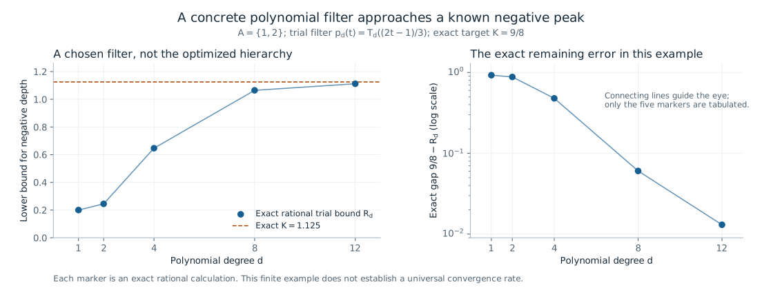 Figure data (JSON) · SVG · PNG
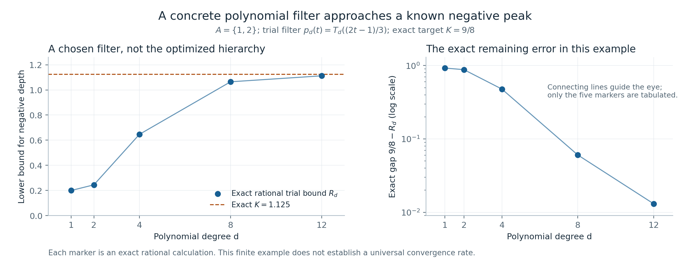
Figure 6. A valid approximation can improve without solving the conjecture. For , an explicitly chosen Chebyshev trial polynomial gives exact rational values at the highlighted degrees, approaching the known depth . These are values of a particular trial quotient , not the optimized hierarchy . The comparison line is an exact minimum in this special example.
This result answers an approximation question for each input. It does not answer the extremal question over all inputs. The degree may be large, exact moments may be expensive to compute, and a generalized eigenvalue calculated in floating point requires an error certificate before being called exact. A finite sufficient degree is not a claim of practical polynomial runtime in the input length.
7. Negative results that narrow the search
Some failed extensions have clean mathematical explanations. Their value is to prevent the same obstruction from being mistaken for progress again.
Unequal amplitudes change the theorem
For weights on , the Fejér-kernel identity gives
and equality is attained. Meanwhile grows linearly in . Therefore the negative depth divided by the coefficient norm tends to zero. Multiplying by gives positive integer weights and the same failure after normalization. Making amplitudes integer-valued does not restore the unit-amplitude conjecture.
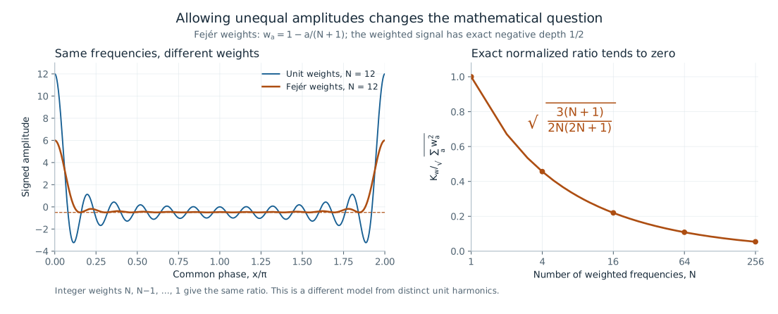 Figure data (JSON) · SVG · PNG
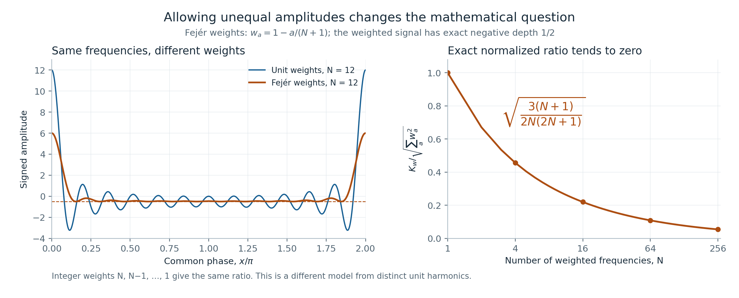
Figure 7. A sharp positive pulse can coexist with a fixed negative floor. Fejér weights give an exact depth of while the coefficient norm grows. The companion normalization plot explains why this is a counterexample to a weighted extension, not to Chowla's original equal-amplitude problem.
A physically inspired weight can emphasize too little
The logistic or Fermi–Dirac-inspired weight , with and threshold fixed at zero, defines a valid lower estimate
For consecutive frequencies, the appendix proves for every . Choosing a larger inverse-temperature parameter cannot turn this particular family into a square-root certificate on every input. An adjustable threshold would be a different family and is not ruled out by this statement.
A promising finite minimum remains finite evidence
Another nonnegative weight is the Riesz product . Its associated quotient can be calculated exactly from integer Laurent-polynomial coefficients. The recorded exhaustive calculation checks all nonempty subsets of . On that finite domain, the smallest normalized quotient is , attained at .
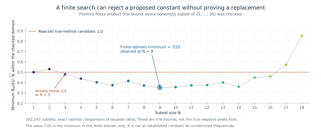 Figure data (JSON) · SVG · PNG
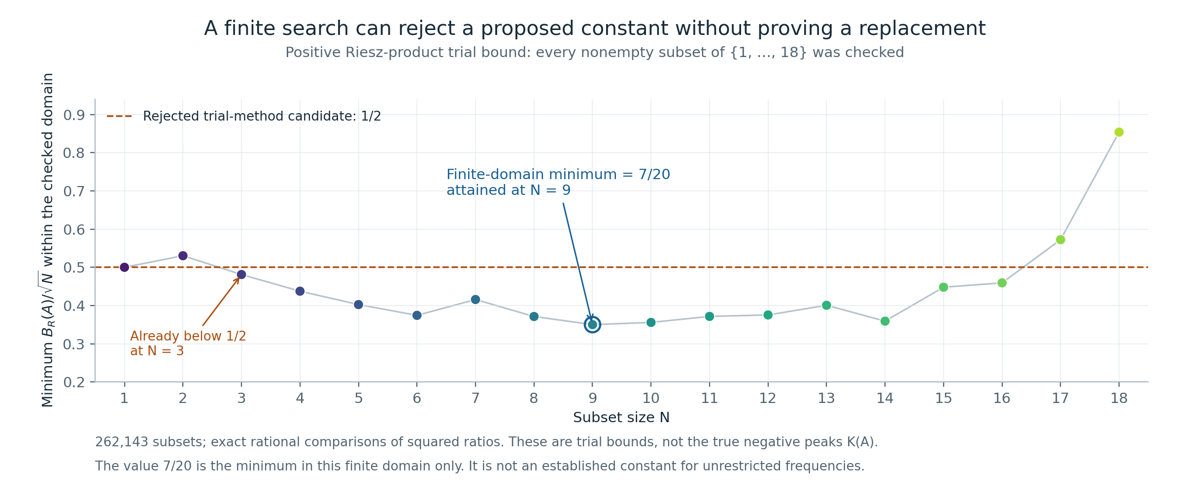
Figure 8. A finite search suggests questions; it does not settle all frequencies. The plotted minima are grouped by set size within the fixed universe . The value is an exact finite-domain result. The rejected candidate fails already for . No universal lower bound for this Riesz quotient is claimed.
8. What the quantum analogy contributes
The wave-to-lattice correspondence is useful because it is exact and preserves the quantity being studied. Other quantum analogies need an equally explicit dictionary. For a harmonic oscillator, a number state has zero mean displacement even when it has nonzero occupation. A coherent state can have a sinusoidal mean displacement, while its mean occupation need not be an integer. The integer spectrum of the number operator does not force the Fourier coefficients of a classical waveform to be integers. Squeezing changes quadrature variances; it need not change the mean waveform. Cappellaro2012 Shapiro6453
Experiments can control individual mechanical quanta, so phonons are physical rather than merely metaphorical. That does not transfer a quantum measurement theorem to a signed classical cosine sum without proof. OConnell2010 In this investigation, the productive question was not whether an analogy sounded surprising, but whether it preserved amplitudes, phases, averaging, and the minimum. The catalogue records where those requirements succeeded and where they failed.
9. Evidence, provenance, and the remaining problem
The companion mathematical appendix supplies full proofs and separates identities, inequalities, and finite examples. The research catalogue indexes ninety numbered approaches and an earlier unnumbered groundwork stage. The archive includes the preserved source notes, code, result files, and three sealed historical archives. It also identifies corrections that supersede earlier statements.
A selected reproduction of the early groundwork checked all nonempty subsets of with two different enumeration procedures. Both found the same unique minimizer of within that finite universe: . Exact certificates put its depth strictly between and . This concerns the actual continuous minimum; the separate Riesz calculation above concerns a particular lower-estimate method. Neither finite result covers arbitrarily large frequencies. The reproduction report and its machine-readable outputs are included in the archive.
There is a material provenance limitation: approaches 41–50 were reconstructed from surviving descriptions rather than recovered as original bytes. In particular, the earlier claim involving 1,980 finite certificates for approach 42 cannot be represented as a reproduced certificate set; those files are missing. A separately available tail argument has a different verification status. These distinctions are documented in the catalogue and provenance notes.
The checks in this project consist of mathematical derivations, exact arithmetic programs, independent calculations within this workflow, and reproducible numerical illustrations. They are not external peer review or formal proof-assistant verification. ChatGPT assisted the writing, derivations, literature comparison, and code preparation. No claim of independent verification by OpenAI is made.
What remains is precise: prove a positive universal lower bound for , or produce a valid sequence of unit-amplitude, zero-phase, distinct positive integer frequency sets for which that ratio tends to zero. None of the weighted examples, finite grids, independent-phase models, or finite searches in this report accomplishes either task. The present contribution is a checked collection of tools and obstructions, with a clear route for readers to inspect and extend the work.
Further reading and supporting material
The accompanying pages are Sampling and Hidden Peaks, Waves and Lattice Particles, Certified Minimum Estimates, The Limits of Wave Analogies, Research Catalogue of Ninety Approaches, and the Mathematical Appendix. Full bibliographic entries appear on the References page. The downloadable research edition includes all of these texts and the reproducibility materials.