
Sampling and Hidden Peaks
A waveform plot is a collection of evaluations joined by a drawing rule. Unless an error estimate is supplied, the lowest visible point is only an estimate of the true trough. A particularly instructive example shows that even an exactly correct RMS calculation cannot repair this gap.
An exact sampling trap
Take , and sample it at the points . The sum of all complex roots of unity is zero at every nontrivial root. Pairing conjugate terms gives
Thus the samples are once and at every other point. Their mean is zero and their mean square is
These are the true continuous mean and mean square. The sample minimum, however, is not the true minimum.
The Dirichlet identity is
with the values at removable singularities defined by continuity. At , its numerator is , so
The final inequality uses for positive . For increasing , the missed depth becomes arbitrarily large even though every nonzero sample remains fixed at .
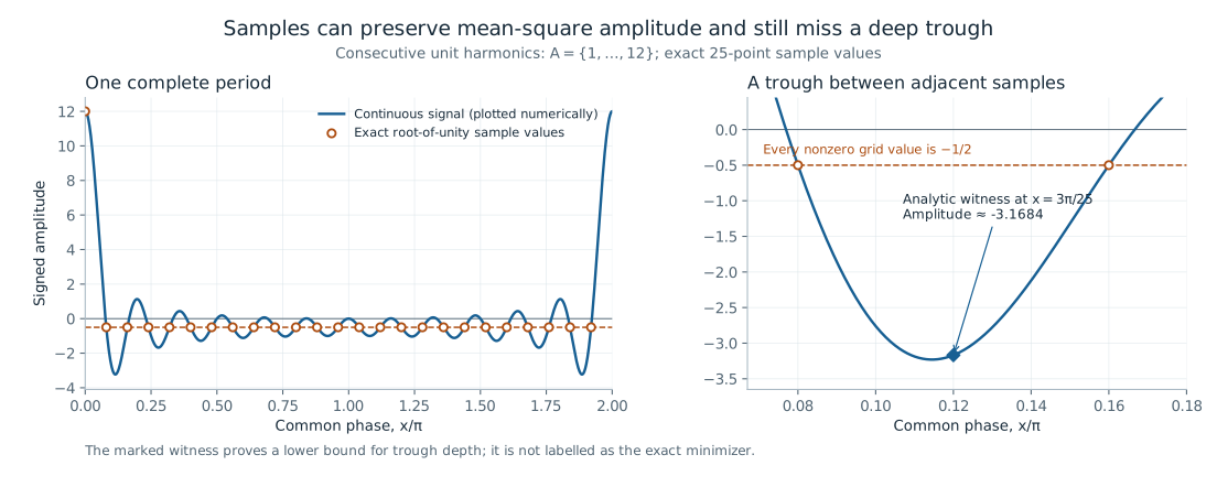 Figure data (JSON) · SVG · PNG
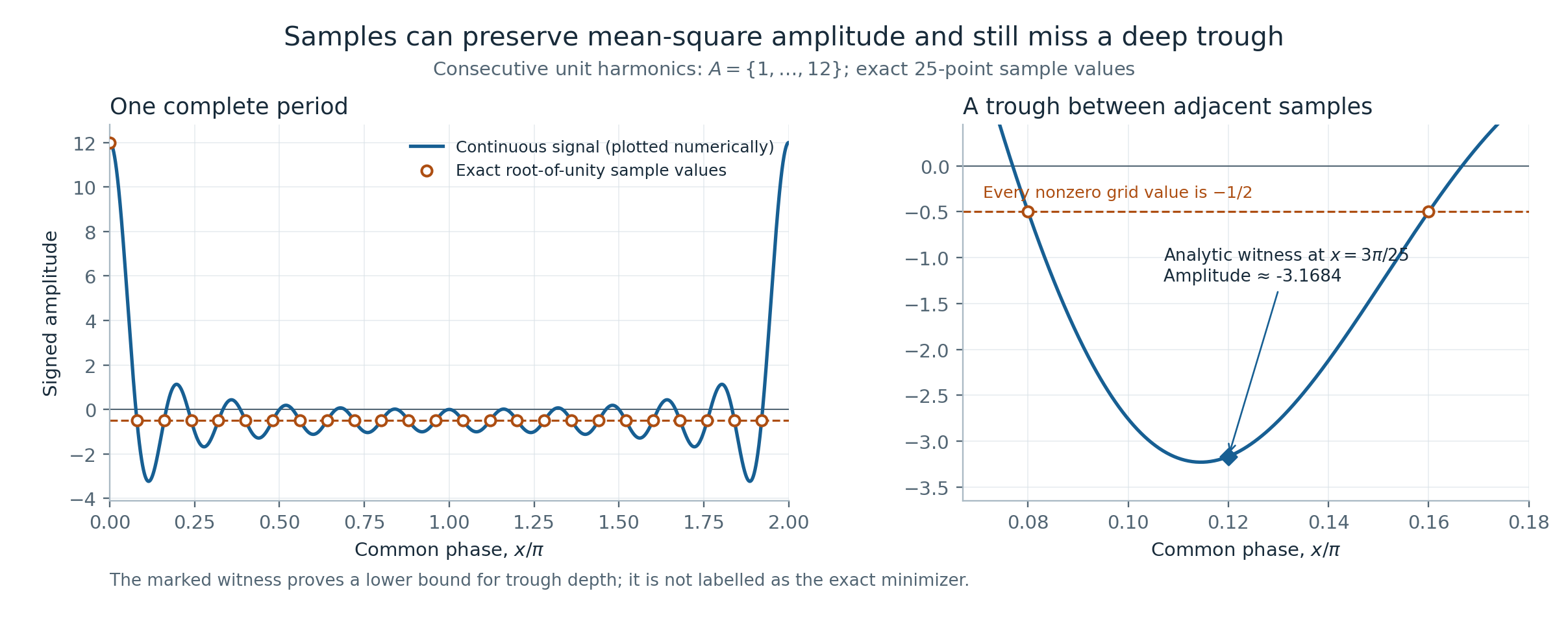
Figure. The default demonstration uses and . The off-grid marker is an exact witness, not an assertion that its location is the exact global minimizer. The continuous line should be labelled as a numerical drawing of the known analytic function.
Explore interactively
Why this does not contradict signal reconstruction
This function has known bandwidth and is a trigonometric polynomial of degree . Its samples determine all of its coefficients. One can reconstruct the polynomial and then minimize it with a separate, controlled procedure. The failure occurs when the smallest recorded sample is treated as the minimum of the reconstructed continuous signal. The information is present, but the operation performed on it is insufficient.
That distinction is useful for a spectrum display or audio-analysis interface. A responsive plot can use a finite grid, but its text should not imply more accuracy than the computation supplies. The same caution applies when a numerical experiment searches many frequency sets: a small observed value of could simply be a trough the grid did not see.
A rigorous interval around a sampled estimate
For a general set , use equally spaced points and define . Every point of the circle is within of a grid point. Since
the true depth lies in . At a true minimizer the first derivative vanishes. Taylor's theorem and , where , also give
These inequalities are exact in real arithmetic. A software implementation must add a numerical evaluation tolerance if it claims a rigorously certified floating-point result. Merely printing many decimal places does not provide that tolerance.
What the interactive version should show
The useful interaction is to move the sample grid while retaining the continuous function and the off-grid witness. A second control changes the number of samples. The readout should distinguish sampled depth, analytic witness, and provable discretization error. When the witness is used, the lower endpoint can be increased to the larger of the sampled value and the witness depth.
The animation should begin only when the reader chooses Play. A paused slider is equally informative and easier to inspect. All states need keyboard controls and a static fallback. There is no reason to request microphone access or play sound: this example explains the geometry of measurement using an ideal mathematical signal.
For a related spectral version, see Waves and Lattice Particles. The full derivation, including the twisted finite ring, appears in the Mathematical Appendix.