
Waves and Lattice Particles
An analogy becomes mathematically useful when it translates the quantity we care about without changing the question. For a cosine sum, a lattice model does exactly that. Its connection to quantum mechanics is informative, but the identity can be understood using shifts and Fourier series alone.
A hopping operator with the same dispersion
Let be the space of square-summable sequences on the integer lattice. Write for the shift of a basis vector. For a finite frequency set , define
The operator permits a hop by each distance in both directions. It is self-adjoint because every forward shift is paired with its adjoint. Under the unitary Fourier transform , it acts as multiplication by
The spectrum of a multiplication operator is its essential range. Here continuity, together with the connected circle and full support of uniform measure, makes this the interval . The lowest spectral value and the most negative wave value are therefore the same number.
This resembles the dispersion relation of a tight-binding model. The analogy concerns a linear operator and its spectrum; it does not assert that a classical audio wave is a stream of localized particles. Standard lattice physics also distinguishes a finite system's eigenvalues from the continuous bands of an infinite periodic system. TongAQM
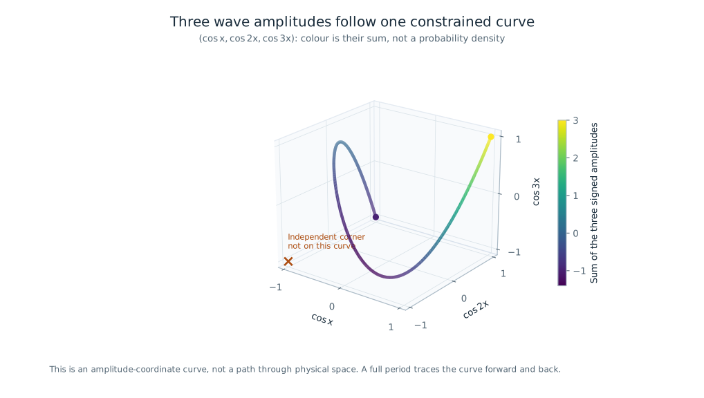 Figure data (JSON) · SVG · PNG
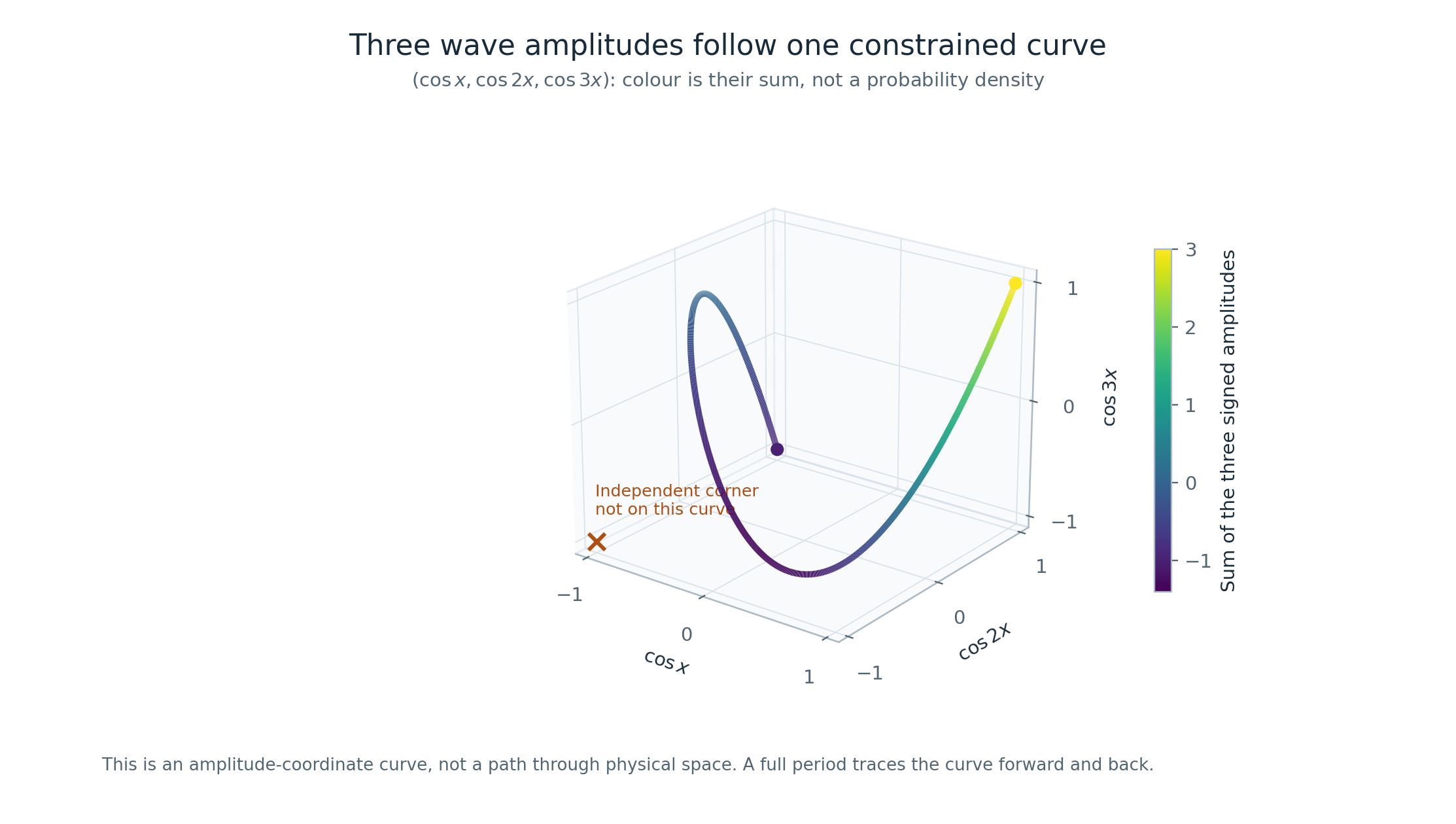
The amplitude-coordinate curve lies on the exact constraints and . Its colour is the sum of its coordinates. The independent corner is not on the curve. A full phase period traces the same curve forward and back. This is not a trajectory through physical space or a quantum probability density.
Explore interactively
A finite ring sees selected phases
On a ring of sites, introduce a phase at the closing boundary. Choose the shift so that . Its eigenphases are , and hence
The untwisted ring samples one grid. Sweeping and all covers a whole period. Consequently,
For and , the untwisted operator is , where is the all-ones matrix. Its eigenvalues are once and with multiplicity . That deceptively shallow lower value is exactly the sampling trap from the companion article. Boundary twisting restores the missing phases. Twisted boundary conditions have an established role in spectral and topological analysis. Bardyn2014
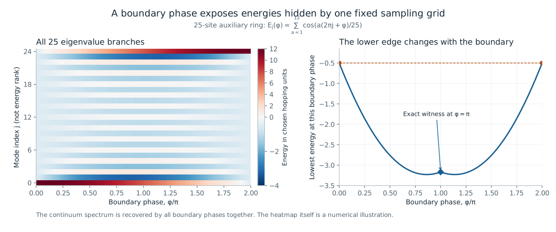 Figure data (JSON) · SVG · PNG
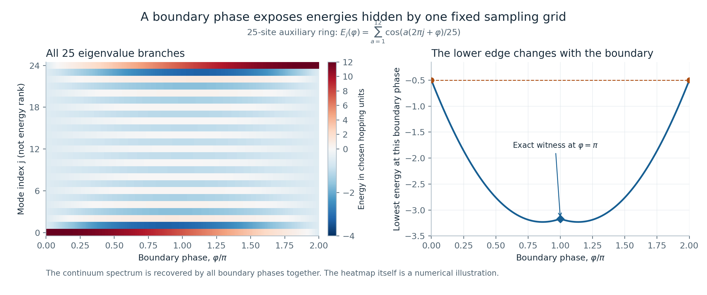
Figure. Each column corresponds to one boundary phase. The colours encode eigenvalue values computed from the explicit cosine formula. An interactive crosshair can show the associated continuous phase on the waveform. Colours represent signed spectral values, not probability or acoustic energy.
Explore interactively
Open boundaries give another approximation
Compress the infinite operator to consecutive sites and call the result . Let . The variational principle gives , and enlarging the box makes these lower estimates nondecreasing. A truncated plane wave supplies the explicit bound
This is a useful convergence statement for a fixed set. It is not uniform in unrestricted frequencies at a fixed box size: if every hop is at least , the compression can have no nonzero entries at all. The finite model then loses the dynamics it was meant to represent. Boundary choices are part of the model, not a cosmetic implementation detail.
Symmetry explains an extreme case
If every frequency divided by their common gcd is odd, a common phase makes every cosine , and . The normalized lattice graph is then bipartite: a hop flips the parity of the site. Its spectrum is symmetric about zero. Conversely, reaching requires all cosines to equal , which forces exactly this parity condition. The appendix proves both directions.
Odd relations between hop lengths obstruct simultaneous anti-alignment. They can provide an upper restriction on how close the minimum can come to . Such an upper bound must not be confused with the lower bound needed for Chowla's conjecture.
The spectral translation is productive because these statements preserve the original minimum. It supplies variational tools, boundary diagnostics, and exact examples. A universal square-root lower bound still needs a further argument about all allowable frequency sets.