
Why a Sampling Grid Can Miss a Waveform’s Deepest Trough
A waveform can be measured at enough points to reconstruct it exactly, yet its lowest recorded sample can still be a poor estimate of its deepest trough. Here is a concrete example: 25 samples give an exactly correct RMS, while the continuous negative peak is more than six times the depth suggested by the lowest sample.
This article, its supporting code, and its mathematical checks were prepared with substantial assistance from ChatGPT. It has not undergone external peer review.
The question grew out of work on Bass Plus, our macOS audio app, and the accompanying Mathematics of Sound project. The example below is an ideal mathematical signal. It is not a measurement of the app or a claim that this estimator is implemented in it.
A small model with a useful distinction
Imagine adding several cosine waves. Each has amplitude one, starts with zero phase, and completes an integer number of cycles during a shared period. For a nonempty set A of distinct positive integer frequencies, write
Here x is phase, measured in radians. To turn it into a time variable, use x = 2πν₀t, where ν₀ is a base frequency in hertz. The values of f are normalized amplitudes, not decibels.
Two different measurements matter. RMS describes the square root of the average squared amplitude. The negative peak describes how far the lowest point falls below zero. Define its depth as
Fourier orthogonality gives a mean of zero and an RMS of √(N/2), where N is the number of frequencies. RMS therefore depends only on the number of unit-amplitude components in this model. The negative peak also depends on which frequencies are present.
For example, the sets {1, 2} and {1, 3} both have RMS 1. Their negative depths are 9/8 and 2 respectively. The first follows by writing cos x + cos 2x as 2(cos x + 1/4)² − 9/8. The second reaches −2 at x = π.
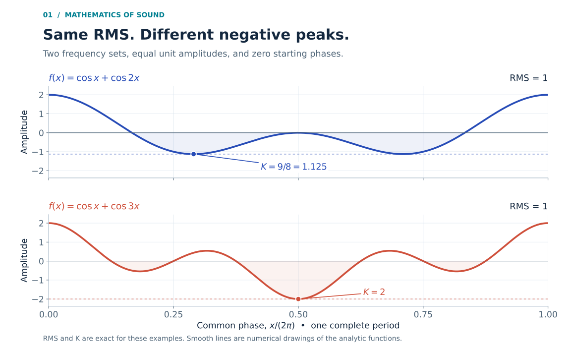
Figure 1. Equal RMS, different troughs. The curves have identical average squared amplitude. Their lowest values differ. The plotted curves are numerical renderings; both stated depths follow from the exact calculations above. Plotting code was prepared with AI assistance.
For an acoustic-pressure interpretation, a negative value means a pressure deviation below equilibrium; it does not mean negative energy. This example also concerns the negative peak specifically. Both signals reach the positive value 2, so their maximum absolute amplitudes are identical.
Twenty-five samples that conceal a deeper trough
Now take every frequency from 1 through N and put q = 2N + 1 equally spaced samples around one period. Include phase zero, and do not duplicate the endpoint at 2π:
At phase zero all components equal one, so the sample is N. Every other sample is exactly −1/2. One way to see this is to sum the q complex roots of unity and pair each root with its conjugate. Equivalently, use the finite Dirichlet-kernel identity
At every nonzero grid point the numerator is zero. The removable singularity at phase zero has the value 2N + 1.
Choose N = 12. The recorded values are 12 once, followed by twenty-four values of −0.5. Their mean is zero, and their mean square is (144 + 24 × 0.25)/25 = 6. Their RMS is therefore √6, about 2.44949: exactly the RMS of the continuous signal.
But look halfway between the first and second nonzero sample positions, at x = 3π/25. The numerator of the identity is −1. The depth at this particular point is
For q = 25, that is about 3.16836. A separate exact rational calculation bounds the true continuous depth between 3.2301038754 and 3.2301038755. The marked point is a convenient witness of a missed trough; it is not the exact minimizer.
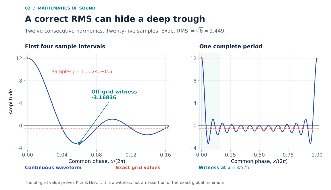
Figure 2. The curve between the samples. The sample markers and the off-grid witness represent different evaluations of the same function. The witness already proves that the sample minimum is insufficient. The exact global-depth check uses a separate polynomial calculation. Plotting code was prepared with AI assistance.
This gap is not restricted to twelve components. Since sin u ≤ u for positive u, the witness depth is at least 1/2 + q/(3π). It grows with N, while the negative depth inferred from the original grid remains 1/2. These are unnormalized sums: their total RMS also grows as more components are added.
The samples contain the information
There is no contradiction with signal reconstruction. A trigonometric polynomial of known degree at most N is uniquely determined by these 2N + 1 samples. Discrete Fourier orthogonality recovers its coefficients.
In physical units, the sample rate is (2N + 1)ν₀, above twice the highest frequency Nν₀. The problem is the operation applied after sampling: taking the smallest recorded value does not minimize the reconstructed curve.
A display that joins the dots with straight lines can consequently give the wrong impression of the trough. Reconstructing the known polynomial, then finding its minimum with a controlled calculation, answers a different and more demanding question.
There is another useful experiment. Move the entire grid by a fraction δ of one sample spacing, using xⱼ = 2π(j + δ)/q. The sampled minimum changes. The sampled RMS remains exactly √6 for every shift in this example: squaring the polynomial produces no frequency as high as q, so averaging over the shifted grid still cancels all nonconstant terms.
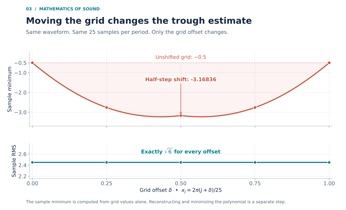
Figure 3. Move the measuring grid, keep the waveform. The offset runs through one sample spacing; offsets zero and one describe the same grid. RMS agreement is exact. The changing sampled-minimum curve is evaluated numerically. Plotting code was prepared with AI assistance.
Explore interactively
The positive peak of the original signal is N at phase zero, and the original grid captures it. This construction demonstrates a missed negative trough; it does not demonstrate a missed maximum absolute peak or an audible defect in an audio product.
Put an error interval around the estimate
The general model also permits a simple bound. On an M-point uniform grid, let Kₘ be the negative of the sample minimum. Define S₁ as the sum of the frequencies and S₂ as the sum of their squares. Then
Why does this work? Every phase lies within π/M of a grid point. The derivative has magnitude at most S₁, which bounds the change in amplitude over that distance. At a true minimum the first derivative vanishes; Taylor’s theorem and the second-derivative bound S₂ give the second, quadratic estimate. Both bounds are valid, so we can use the smaller one.
The bound applies to any finite frequency set in this model, and also to a shifted uniform grid. It is conservative. For a fixed set, doubling M reduces the quadratic allowance by a factor of four; it does not guarantee that every observed error decreases by exactly that factor. On a very coarse grid, Kₘ can even be negative, so the definition matters.
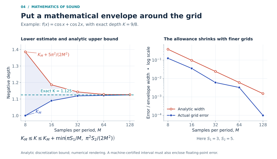
Figure 4. An estimate with a stated allowance. For A = {1, 2}, the exact answer is 9/8. Each interval starts at the sampled estimate and adds the analytic discretization bound. Its displayed endpoints are floating-point approximations of mathematical bounds. Plotting code was prepared with AI assistance.
Try the calculation
This small example uses only the Python standard library:
from math import cos, pi

A, M = (1, 2), 32
samples = [sum(cos(2*pi*a*j/M) for a in A) for j in range(M)]
k_grid = -min(samples)
s1, s2 = sum(A), sum(a*a for a in A)
error = min(pi*s1/M, pi*pi*s2/(2*M*M))

print(f"Approximate interval: [{k_grid:.9f}, {k_grid + error:.9f}]")
print("Exact depth for this example: 9/8 = 1.125")
The approximate interval is [1.118969855, 1.143065568]. It contains 1.125, as the analytic argument predicts.
There are two sources of error to distinguish here: missing a minimum between grid points, and rounding while evaluating numbers. The formula controls the first. Ordinary floating-point cosine evaluations do not automatically certify the second. A machine-certified interval needs justified evaluation-error bounds and outward rounding, or an exact alternative such as the rational polynomial check supplied with this article.
What to carry into an audio interface
A useful analysis display can show the sampled minimum, identify any reconstructed curve, and state an error allowance when one is available. A slider that moves the sample grid makes the distinction visible without changing the underlying waveform. The axes should retain the same amplitude scale throughout the interaction.
This is an educational example using equal-amplitude integer harmonics. It does not establish how arbitrary music, different phases, a playback device, or a processing chain behaves. It also does not resolve the open cosine-sum question that motivated the wider project. Its practical contribution is narrower: a correct average can coexist with a poor extremum estimate, and a small amount of analysis can make that uncertainty explicit.
Attribution and reproducibility
The Fourier-series and Parseval background is standard; see the NIST Digital Library of Mathematical Functions, §1.8. The Chebyshev identity Tₙ(cos x) = cos(nx), used in the accompanying exact polynomial check, is given in §18.5, equation 18.5.1. These classical tools and the elementary bounds above are not claimed as new discoveries.
The reproducibility files contain the plotting code, the standard-library demonstration, and an exact rational verifier. The verifier forms the polynomial sum of T₁ through T₁₂, isolates every critical point using Sturm’s theorem, and bounds their values. This checks the twelve-component example; it is not external peer review or proof-assistant formalization.
Project affiliation: CliDeck Research Notes, Mathematics of Sound. This is educational material authored for the project that motivated the investigation.